Luckily, Sheets supports custom functions and formulas that help make up for some of these shortcomings. If users are savvy with formulas or can do a little bit of scripting, Sheets can be as powerful as they make it. One particular functionality that Sheets doesn’t natively support is the ability to find duplicates in Google Sheets – whether it’s duplicate data in cells or rows. While there is a way to quickly remove duplicate entries, using the Remove duplicates option under the Data menu, there’s no way to only isolate those duplicates. The good news is that there is a way to accomplish this. In this article, let’s go over how to find duplicates in Google Sheets by taking advantage of conditional formatting.
What Is Conditional Formatting In Google Sheets?
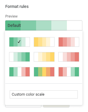
Conditional formatting is a feature present in many spreadsheet editors which allows the user to apply text-based and other visual formatting to a cell based on certain conditions. For example, a user may be recording their monthly budgeting using a spreadsheet, wanting to know at a glance if they go over a $500 spending limit. In the spreadsheet column where the total for the month is tallied, a conditional formatting rule can be set to bold rows with a value over $500, making it easy to see where this occurred. In Google Sheets, conditional formatting allows users to apply formatting based on a long list of preset rules or by entering a custom formula. The formatting style changes available include bold, italics, underline, strikethrough, text color, and cell color. Additionally, users can use a color scale, instead of a single color, and define a minimum and maximum value, and their respective colors, for automatic color scaling.
How To Use Conditional Formatting to Find Duplicate Rows In Google Sheets
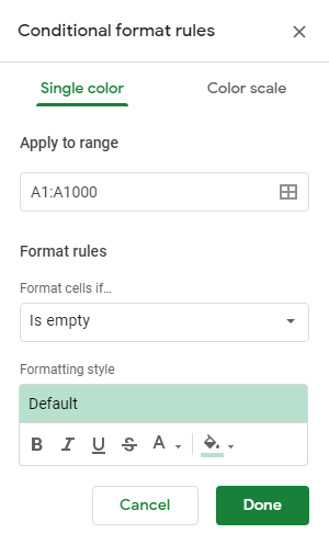
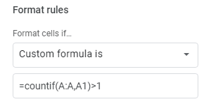
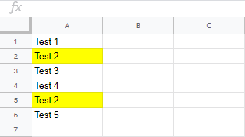
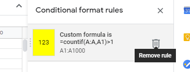
For anyone working on a lengthy sheet of data, duplicate entries can become a problem that will sometimes break the flow of things. Users may not simply want to delete this data, which Sheets natively supports, and instead analyze and work with it. Using a custom formula with conditional formatting, this is possible. The first step to achieve this is to highlight the entire column that needs to be searched for duplicates by clicking on the column label above it. Once highlighted, right-click and select Conditional formatting. This will bring up a panel on the right side of the window that shows conditional formatting rules. The column range selected will be prefilled in the Apply to range field, so that won’t need to be touched. Next, you want to click on the dropdown menu beneath Format rules to change this condition to Custom formula is. A text field will appear beneath the dropdown menu after this is done, and the following formula should be entered: =countif(A:A,A1)>1 However, it will need to be modified to replace all instances of “A” with the column letter that is being searched for duplicates in Google Sheets, which will be shown in the Apply to range field. The final step is to set the formatting to apply to all cells in this row that contain data found more than once. If working with a large set of data, the best formatting to set might be a fill color. Using it, a bright and noticeable color such as yellow, hot pink, or lime green will really stand out and allow for noticing duplicates at a glance while scrolling. Now, all rows that contain data that is found in at least one other row will be highlighted or formatted in whatever way was chosen. If duplicate rows are deleted, the single row remaining will have its conditional formatting removed automatically. One might ask, “Why go through this trouble when Google supports duplicate removal in two simple clicks?” Well, this system is inflexible and imperfect. For example, there is no way to change which duplicate is deleted. Some users may want the first instance deleted, and others the last—Google gives no option and removes all duplicates but the very first. Using this simple conditional formatting rule, the user is in complete control of managing duplicates in a way that won’t risk breaking their sheet. Best of all is that conditional formatting is entirely dynamic, so you’ll never need to remove formatting if you choose to remove all duplicates in some way. However, should the conditional formatting rule ever need to be deleted, it’s as simple as clicking on the Format menu and then Conditional formatting, which will show the same right-side menu as before. Users can hover their cursor over the row that shows the custom formula we’ve just created and click on the trash can icon that appears to remove it. When Google Sheets’ native option to find duplicates to remove them just isn’t powerful enough or scrambles data in a way that can’t be afforded, the simple custom formula highlighted in this article allows users to take matters into their own hands. Do you have any questions or comments about using this conditional formatting rule? If so, please leave us a comment below.

